
Simulation using a SPICE simulator (Simulation Program with Integrated Circuit Emphasis) is handy for checking out designs before building them as well as helping to understand designs and circuit problems. You can experiment without blowing anything up! LTspice from Linear Technology is particularly useful as it is free and available to download from their web site. While there are “better” SPICE simulators out there, they are all based on the same principles and the results you will get from the same models and circuits with be identical with LTspice. Also, it is the only way you will be able to simulate some of Linear Technology’s chips, such as power supply ICs. They don’t supply standard SPICE models for those – only their own format subcircuit models in binary format. So, even if you have another SPICE simulator (which I do), you may want to use LTspice anyway from time to time for simulating their power supply ICs. The approach taken by Texas Instruments is different – they supply encrypted PSpice models instead – fine if you use PSpice, useless if you don’t!
The easy way to first use LTspice is using one of the “jigs”. These are schematics already drawn for many of the Linear Technology ICs so you can use them as a quick starting point. So, if you want a switching regulator (boost) to generate 12V at 1A from 3V and choose the LTC1872, simple open the file 1872.asc under the “examples\jigs” directory in the LTspice installation. You will see the following schematic:
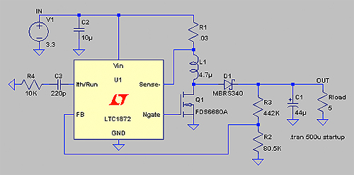
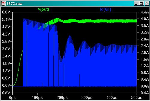
While this might not be exactly the circuit required for your application (it is for 5V at 1A), you can still use it as a starting point and edit the components/values to suit your design. For now, simply select “Simulate | Run” from the menu. A graph window will open and probably nothing will be shown. That is the results plot window and you first need to select some results to show. If you hold the cursor over the wire labeled OUT the cursor will change shape to a “probe” – click on the wire with that probe and you should see something like this:

This shows the results of the simulation i.e. the voltage on the output node as the circuit starts up. You can zoom in on the waveform to show the output ripple. You can plot currents – for example hold the cursor over the load resistor Rload and the cursor will change again allowing you to plot current. Hold it over the transistor drain and it will allow you to plot drain current.
Keep an eye on the lower part of the screen because handy information is shown as you move the cursor around. Also, try the ALT key and the look at the bottom of the screen – it will let you know that you can plot power dissipation. Similarly, it often gives information about whether to left click or right click but even if it doesn’t, a right click is required for some functions. A right click is required to edit a component, not a left click. A left click usually plots results.
If you get too many plots on the screen you can right click a label (e.g. V(out) shown above) and the “Expression Editor” popup will give you the option editing the equation or color but also the option to delete the trace. The “help” is quite good with a useful run through the features under “contents”, an explanation of the basic circuit elements and SPICE commands as well as a search.
Coming from other SPICE simulators can take a bit of getting used to but the simulation command (transient in this case) is shown on the schematic and can be edited by either right clicking on it – the “.tran 500u startup” text or selecting “Simulate | Edit Simulation cmd” from the menu.
If you want to move, delete or add components, they are under the “Edit” menu. If you want to learn more about SPICE netlists and understand more of what is going on behind the schematic, you can look at the netlist using “View | SPICE Netlist”:
* C:\Program Files\LTC\LTspiceIV\examples\jigs\1872.asc
L1 N001 N004 4.7µ Rser=0.02 Rpar=5000
V1 IN 0 3.3 Rser=.1
C1 OUT 0 44µ Rser=.1
C2 IN 0 10µ Rser=0.02
C3 N003 N002 220p
R1 IN N001 .03
R2 N005 0 80.5K
R3 OUT N005 442K
R4 N002 0 10K
D1 N004 OUT MBRS340
Rload OUT 0 5
XU1 N003 0 N005 N001 IN N006 LTC1872
M§Q1 N004 N006 0 0 FDS6680A
.model D D
.lib C:\Program Files\LTC\LTspiceIV\lib\cmp\standard.dio
.model NMOS NMOS
.model PMOS PMOS
.lib C:\Program Files\LTC\LTspiceIV\lib\cmp\standard.mos
.tran 500u startup
.lib LTC1872.sub
.backanno
.end
Here you can see each of the elements used in the simulation. Before companies added graphical front and back end processing to SPICE the netlist was what you had to work with. While it would seem that you can avoid learning about the netlists, when you have a problem it can be useful to look at them and also when importing models from other sources you may have to do a little tweaking to correct some of the syntax differences between different SPICE implementations. Most SPICE simulators have deviated from the “standard” SPICE and modified it and the way these have been done varies from simulator to simulator. For example a MOSFET model for HSPICE called LEVEL49 is called LEVEL7 in PSpice. The syntax of some of the controlled voltage sources differs between simulators.
You are not restricted to just using LTspice models. If you have a SPICE model from another manufacturer then you can add it to LTspice provided it is not encrypted and create a symbol for it (or re-use an existing symbol if it is standard, such as an opamp). Also, remember to look in the “Examples\Educational” directory.