It’s not enough to model and simulate circuit behavior – you also have to investigate the effects of component variations from their nominal values due to unavoidable tolerances.

There’s a semi-serious quip that scientists can build one of anything – but just one; it takes engineers and production experts to build it again and again and again. That quip doesn’t apply only to scientists, of course; it applies to engineering prototypes, and short pilot runs as well. It’s often a real-world shock to new engineers just out of school when they have to get a product qualified for production beyond just doing a demonstration of one working unit or even that small pilot run.  Now, “hand crafting” of each unit is no longer a viable approach, and the accumulation of component tolerances and drifts means that some of the production units may not work to spec or at all.

What magnitude of tolerances are we looking at? Standard resistors can be ±5%, ±10%, or ±20% (depending on the type and ordered version), while capacitors can be ±20% and many standard-grade electrolytic capacitors can range anywhere from -20% to +80%. Note that these are just initial tolerances and don’t consider thermally induced drifts or component aging.  The tolerance issues primarily affect analog components ranging from sensors to basic transistors to analog front ends and even power-related components such as voltage references and MOSFETs; digital components are less sensitive initially.

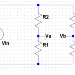
Many years ago, I had the privilege of listening in while the late (and sorely missed) analog guru Bob Pease gave a basic “back of the envelope” introduction to the realities of analog-circuit design to some visiting students, using a single-transistor amplifier circuit similar to Figure 1. He said the circuit as shown would work fine, then walked through the consequences of tolerance variations of each individual component, including the transistor beta (which could range over a 2:1 ratio). The circuit still worked but deviated from its nominal gain as each component was “dithered” over its range.

Then he took it a step further and simultaneously varied the values of two, then three of the components – and pretty soon, the circuit would no longer work. That, he said, is reality when going from a benchtop single-unit demonstration into a volume-production environment.

Obviously, this sort of manual analysis isn’t practical for designs with dozens or even hundreds of components with different tolerances and circuit sensitivities. If you think about it, it’s amazing that anything works at all, as the odds of tolerances and drifts stacking up against it are pretty high.

The obvious way to understand the severity of the problem is to do a worst-case analysis using each component’s extreme high/low values. However, it’s often hard to really discern what “worst case” means in a complicated circuit: for one component, it may be a value at the high end of its range; for another, it may be the low end. Also, there is an interplay among presumed worst-case values since an extreme of one component’s value may aggravate the problem when combed with another component’s worst-case value or may, in fact, counterintuitively moderate it. Pretty soon, you have an intangible, impossible-to-analyze set of equations.

Fortunately, there are powerful tools available to deal with this situation. Among them is what is referred to as “Monte Carlo” analysis, which is well-suited for the strength of computers and software. In this approach, the values of all components are randomly varied while thousands of simulations are run on the circuit model (using Spice or other). These runs can flag those combinations of component values for which performance falls below an acceptable threshold or fails entirely.

The designer then looks at the specific components and associated values which caused this outcome and decides how to deal with it. Options include tightening up the allowed tolerance of the components as listed on the bill of materials (BOM), going from, say, a ±10% value to a more costly but reassuring ±5%; adding some sort of manual or automated electronic trim to the circuit (digital potentiometers – “digipots” – are well-suited for this), or, in a worst-case, redesigning that part of the circuit to be less sensitive, via an alternate topology such as a ratiometric Wheatstone or differential configuration rather than absolute-value approach.

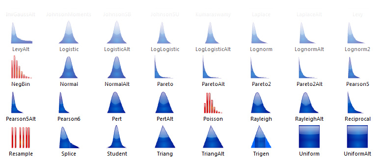
A logical issue when doing these Monte Carlo simulations concerns the probability distribution of the tolerance values for the various components. Most programs allow the user to select a profile for each component range, such as a simple uniform, normal (Bell) curve, or a more advanced distribution (Figure 2).

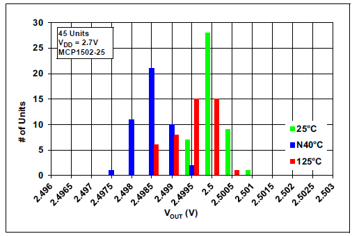
Using the appropriate distribution function for each component can also provide insight into additional perspectives, such as the likelihood of the various outcomes and sensitivity to variations of a given component. An experienced component engineer can advise which profile makes sense; some vendors include this data on their datasheets, often in the form of a histogram, as shown by the Microchip MCP1502 voltage reference (Figure 3).

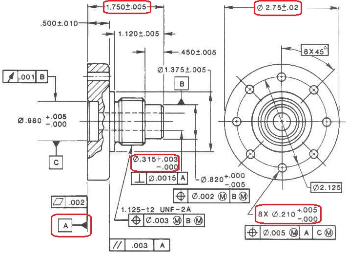
It’s not just electronic circuits and systems that benefit from Monte Carlo simulation; mechanical designs also use it. Fabrication drawings and specifications state nominal dimensions plus minimum and maximum dimensional tolerance, and in many cases, the “plus” and “minus” tolerances are not the same value (Figure 4). Monte Carlo analysis is also used for risk assessment and quantitative analysis in disparate fields such as finance, project management, manufacturing, basic research and development, and more.

Conclusion

Analysis and simulation based on the realities of component tolerance and imperfections separate a possibly good design from a  credible implementation. You either do it up-front as part of the pre-production process and sleep well, so to speak, or you do it afterward in a crisis mode, put in long days and nights, incur severe delays and costs – and all with a severe ripple effect on getting product out the door and shipped.

EE World Related Content

Wheatstone bridge, Part 1: Principles and basic applications
Wheatstone bridge, Part 2: Additional considerations
Transistor circuit configurations and Spice
When you can use Spice and its variants, when you can’t
New Standard Interface for Advanced SPICE capabilities handles complex physics for digital, RF designs
SPICE: how to choose an analysis

References

Palisade Company, Various relevant article
Microchip Technology Inc, “MCP1502 High-Precision Buffered Voltage Reference Data Sheet”