There are many ways to implement the automatic gain control function, which is critical to the proper performance of many wireless and other links.
The automatic gain control function has been embedded in radio links since the earliest days of wireless technology, but the need for AGC is not limited solely to that application. Along with its optical sibling of automatic power control (APC), AGC allows circuits to handle signals that inherently and unavoidably have a wide and uncontrolled dynamic range and optimally match the signal range to the capabilities of the circuit and system.
This FAQ will look at why AGC is needed, where it is used, how it is implemented, and some associated issues.
Q: What is AGC?
A: it is a scheme by which the strength of an incoming signal from a communications channel is assessed, and the gain of the analog front end (AFE) which captures this signal is dynamically adjusted to make that signal “fit” into the maximum or near-maximum range of the AFE amplifier, (Figure 1). In this way, the dynamic range and signal-processing performance of the input stage and amplifier are optimally used.
Q: What are the key functional elements of an AGC?
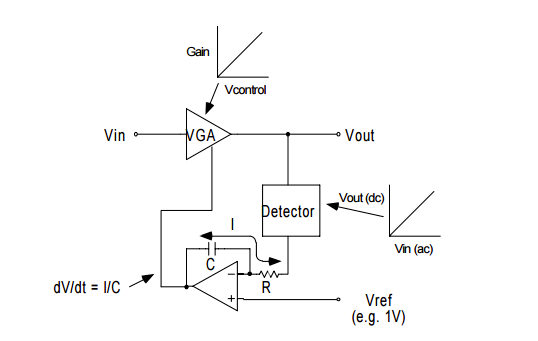
A: At its core, the AGC function consists of two elements: a detector that assesses the received signal amplitude (voltage or power) and an amplifier whose gain is controlled by this detector.
Q: Is AGC an analog function?
A: With very few exceptions, it is. There are some special cases where the AGC function is mainly accomplished but not entirely using digital techniques. However, most applications must be done using analog techniques due to signal range, bandwidth, or power-dissipation constraints.
Q: What is the channel problem for which AGC is needed?
A: The problem is most apparent but not limited to wireless RF channels. For long-distance wireless links, there are continual received signal strength (RSS) changes due to fading, multipath, movement of the source and/or receiver, and propagation variations, all of which cause the received signal strength to vary over a wide range, even if the source transmitter power is constant. Even for shorter-distance channels such as a local Wi-Fi network, there are channel variations when someone steps between the source and receiver antennas or when one or both antennas are mobile.
Q: Is AGC a relatively new function?
A: Not at all. The need for it was recognized in the early days of wireless, and clever schemes using vacuum tubes were developed to implement it. Now, it is done with discrete transistors (in some cases) or application-specific ICs (in most cases); the latter offers superior performance, consistency, and accuracy at lower cost and space.
Q: Does this RSS variation only affect RF wireless links?
A: No, it also can affect optical links such as free-space optical communications and even optical-fiber channels when there are longer-term, slower variations as temperature changes, the fiber moves or bends, or operating parameters shift. These and other non-RF scenarios will be discussed in the final part of this article.
AGC is also needed in applications such as radar, where the return signal strength is a function of uncontrollable, unknown factors such as the target radar cross section (RCS) and distance to target. Keep in mind that the path-loss signal strength follows the inverse square law and drops off as the square of that distance; in the case of radar, it is a two-way trip, and so there is a double path loss. The same scenario applies to sonar, which is “wireless” although not RF.
Q: What is the magnitude of these variations?
A: It depends on the situation, of course. A highly localized system may see variation over a modest power ratio of 10:1 (10 dB). In contrast, a long-distance link or radar return can easily see variation over many orders of magnitude. RSS variations of 40-60 dB (40 dB = 10,000:1 power ratio) are not unusual in these cases, as many factors can combine and add up: antenna movement, propagation variation, rainfall, and more.
Q: So what’s the problem? If the signal is low, just increase the gain of that first stage, and those low-level signals will be amplified to the maximum and thus recoverable.
A: Yes, they will, but what happens when the signal magnitude increases by a factor of “just” ten or even tens of dB? The front-end amplifier then overloads, goes into saturation, and can no longer amplify. Instead, it locks up, distorts severely, or does other bad things. In effect, the front end is useless until the signal comes back into the normal operating range.
Q: OK, so what about using the opposite solution: why can’t you limit the gain so that even the strongest signal does not overload the front end?
A: Yes, you can do that, but that means that weak signals will be almost imperceptible or below the noise floor of the front end and so be irretrievable. Either way, attempting to optimize range and signal recoverability despite wide swings in received signal strength is a problem.
Q: So what does AGC do, and how does it do it?
A: An AGC circuit continuously assesses the signal strength, but not the details (information or data), and dynamically adjusts the gain to maintain the match between the received signal strength and the useful input range of the analog front end. This applies to analog and digital signals: a properly designed AGC function can significantly improve bit error rate of a channel with RSS variations and noise.
Q: It all sounds easy enough, but is it?
A: Yes and no. There are many ways to do it, but the details of the AGC control loop – and it is a closed loop – must be matched to the dynamics of the input signal as well as its modulation type (AM, FM, pulse, and others). Further, the AGC specifics vary with the channel itself, as the needs of a short-range Wi-Fi connection differ from a local cellular link, from a worldwide radio link, and even a satellite link (low Earth orbit, medium Earth orbit, and geostationary orbits all have large differences in the variations of their RSS).
Q: Is that all?
A: No. Among other parameters, the speed with which the AGC acts and responds is a factor; these are called AGC attack and decay times. As with all closed-loop systems, there’s a balance between speed of response, overshoot, stability, and even possible oscillation. The attack and decay times must be compatible with the nature of the RSS variations, the signal type, and the modulation. A pulsed signal, such as from radar, needs very different attack and decay times compared to a broadcast AM signal.
Q: What is “gain pumping?”
A: If the attack/decay times are too fast, the system gain will increase and decrease too quickly for the application. This gain-pumping can make signal demodulation difficult and degrade system performance. Again, AGC loop dynamics must be matched not only to the signal range but also to the application type, bandwidth, and modulation.
Q: Is there are other use for the AGC circuit?
A: If the system is precisely scaled, the control voltage can also be used as a measure of the input signal magnitude and help the user optimize the receiver parameters, siting, or antenna alignment. The AGC control voltage is then used as the received signal strength indicator (RSSI).
The next part of this article will look at specific approaches to implementing the AGC function.
Related EE World content
How does a precision rectifier work?
Digipots as electronic potentiometers, Pt 3: Enhancements
Analog computation, Part 1: What and why
Analog computation, Part 2: When and how
RMS power detector operates up to 30 GHz
Why use a nonlinear amp?
Stanford researchers build earthquake observatory with optical fibers
RF over fiber: overcoming an inherent transmission-line problem, part 1
RF over fiber: overcoming an inherent transmission-line problem, part 2
Free-space optical links, Part 1: Principles
Free-space optical links, Part 2: Technical issues
Free-space optical links, Part 3: Standard units
Undersea optical-fiber cables do double-duty as seismic sensors, Part 1: Context.
Undersea optical-fiber cables do double-duty as seismic sensors, Part 2: Application
External References
AGC for wireless and other channels
- All About Circuits, “Understanding Automatic Gain Control”
- Science Direct, “Automatic Gain Control” (shows its use in various non-wireless applications)
- Analog Devices, “Design and Operation of Automatic Gain Control Loops for Receivers in Modern Communications Systems”
- Analog Devices, “AD8368 800 MHz, Linear-in-dB VGA with AGC Detector”
- Analog Devices, CN3090, “20 GHz to 37.5 GHz, RF Automatic Gain Control (AGC) Circuit”
- Analog Devices, “Chapter VIII: Design and Operation of Automatic Gain Control Loops for
Receivers in Modern Communications Systems” - Analog Devices, “Stable, Closed-Loop, Automatic Power Control for RF Applications AN-1507”
- Analog Devices, “Measurement and Control of RF Power (Part I)”
- Analog Devices, “Measurement and Control of RF Power (Part II)”
- Analog Devices, “Measurement and Control of RF Power (Part III)”
- net, “Automatic Gain Control (AGC) in Receivers”
- Electronics Notes, “Superhet Radio AGC – Automatic Gain Control”
- EETimes, “Wireless 101: Automatic Gain Control (AGC)”
AGC in Wein-bridge oscillators
- Worcester Polytechnic Institute, “Wien Bridge Oscillator: Automatic Gain Control (AGC)” (lab project with analysis)
- Wikipedia, “HP 200A” https://en.wikipedia.org/wiki/HP_200A (light bulb as PTC resistor)
- Hewlett-Packard, “Schematic for Success: The HP200A” (schematic with specifics and bulb)
- Hewlett-Packard, “A real gem: HP’s audio oscillator patent turns 60” (HP 200 history)